
An application of Simulated Annealing
My wife has a perennial problem. Working at a university every year she has to assign some 200 students to 20 thesis supervisors. With Excel as her only tool and many matchings, an unthankful task. Time for writing a Machine Learning program.
Each student is given two choices from twenty supervisors. The totals of all student’s first choices (blue bars) and second choices (orange bars) are shown in the top row figures. The twenty supervisors are indicated by the letters A through T.
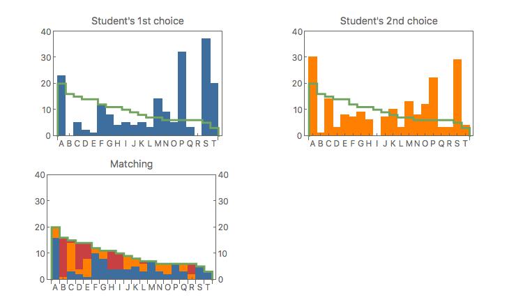
Some supervisors are very popular but have only a few openings. The availability of supervisors is shown by the green line. The total counts under the green line are the same as the total counts of the blue and orange bars.
The discrepancy between the green line and the blue or orange counts shows the imbalance between the demand (by the students) and the supply (by the supervisors). How can one make a fair assignment?
A naive attempt is to start at the top of the list of students and assign them to the supervisor of their first choice. After a number of matchings, some supervisors have ran out of openings and the next student’s first choice cannot be honoured anymore. This student is then matched with her/his second choice.
At some point down the list also no second choices can be matched anymore. Then this student is matched with an arbitrary supervisor. This naive type of matching is rather unfair to the students at the bottom of the list. They will almost certainly be poorly matched. Unnecessarily.
The Simulated Annealing computing method is ideal for this task. This early example of Machine Learning was invented by Nicholas Metropolis and other scientists in the 1950s. The key idea is to randomize the assignment problem.
The program starts with assigning every student randomly to a supervisor. Every assignment is valued by a distance. A first choice match gets a distance of 1, a second choice match a distance of 2, and a mismatch get a distance of 7. The total sum of all the distances measures overall quality of the matching. The smaller this sum, the better the matching.
Next, randomly, two student-supervisor combinations are taken, the two supervisors are interchanged, and the new student-supervisor distances are compared with the old ones. When the sum of both distances is smaller the new match is accepted. When the sum of the distances is bigger, the interchange is a deterioration and is usually rejected. One trick of the trade in Machine Learning is that a small fraction of deteriorations is accepted anyway. Contrary to one’s intuition, this improves the overall result in the long run. Thanks to Metropolis et al.
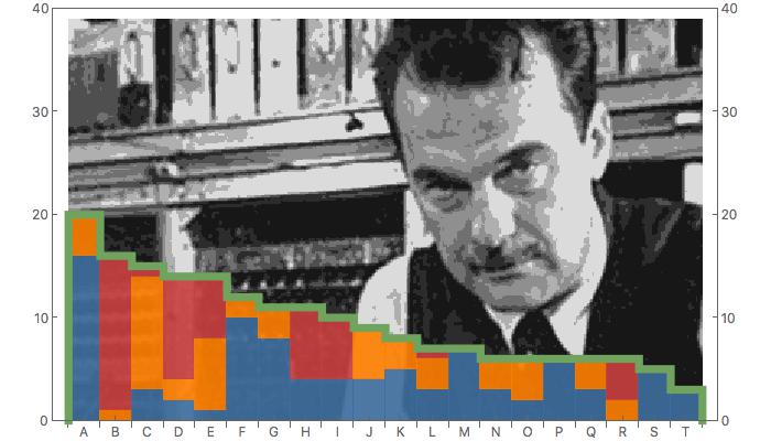
Nicholas Metropolis overseeing our result.
In my wife’s case, this long run is a mere sixty-thousand interchanges. In the first few thousand interchanges improvements are plentiful, but later on they become more rare. When the sum of the distances does not decrease anymore, a “close packing” of student-supervisor combinations has been obtained.
The best matching result is shown at the bottom figure. The supply and demand are matched exactly. For each supervisor the mix of student preferences can be read off. The blue segments are the first choices, the orange segments the second choices, and the red segments are the remaining ones. In total 46% of first choices (total blue area) are accommodated, 28% of the second choices (total orange area), and 26% as remainders (total red area).
By rerunning the program a number of times, we have gained confidence that better solution will be very difficult to find. Student and supervisors have to make due with what we have presented here. Most importantly, every student got the same fair chance of being assigned to her/his supervisor choice.